8
Prediction
Tidy Data Science with the Tidyverse and Tidymodels
W. Jake Thompson
https://tidyds-2021.wjakethompson.com · https://bit.ly/tidyds-2021
Tidy Data Science with the Tidyverse and Tidymodels is licensed under a Creative Commons Attribution 4.0 International License.
Your Turn 0
- Open the R Notebook materials/exercises/08-prediction.Rmd
- Run the setup chunk
01:00
(Applied) Data Science
AmesHousing
Descriptions of 2,930 houses sold in Ames, IA from 2006 to 2010, collected by the Ames Assessor’s Office.
# install.packages("AmesHousing")library(AmesHousing)ames <- make_ames() %>% dplyr::select(-matches("Qu"))ames contains descriptions of 2,930 houses sold in Ames, IA from 2006 to 2010. The data comes from the Ames Assessor’s Office and contains things like the square footage of a house, its lot size, and its sale price.
glimpse(ames)#> Rows: 2,930#> Columns: 74#> $ MS_SubClass <fct> One_Story_1946_and_Newer_All_Styles, One_Story_1946…#> $ MS_Zoning <fct> Residential_Low_Density, Residential_High_Density, …#> $ Lot_Frontage <dbl> 141, 80, 81, 93, 74, 78, 41, 43, 39, 60, 75, 0, 63,…#> $ Lot_Area <int> 31770, 11622, 14267, 11160, 13830, 9978, 4920, 5005…#> $ Street <fct> Pave, Pave, Pave, Pave, Pave, Pave, Pave, Pave, Pav…#> $ Alley <fct> No_Alley_Access, No_Alley_Access, No_Alley_Access, …#> $ Lot_Shape <fct> Slightly_Irregular, Regular, Slightly_Irregular, Re…#> $ Land_Contour <fct> Lvl, Lvl, Lvl, Lvl, Lvl, Lvl, Lvl, HLS, Lvl, Lvl, L…#> $ Utilities <fct> AllPub, AllPub, AllPub, AllPub, AllPub, AllPub, All…#> $ Lot_Config <fct> Corner, Inside, Corner, Corner, Inside, Inside, Ins…#> $ Land_Slope <fct> Gtl, Gtl, Gtl, Gtl, Gtl, Gtl, Gtl, Gtl, Gtl, Gtl, G…#> $ Neighborhood <fct> North_Ames, North_Ames, North_Ames, North_Ames, Gil…#> $ Condition_1 <fct> Norm, Feedr, Norm, Norm, Norm, Norm, Norm, Norm, No…#> $ Condition_2 <fct> Norm, Norm, Norm, Norm, Norm, Norm, Norm, Norm, Nor…#> $ Bldg_Type <fct> OneFam, OneFam, OneFam, OneFam, OneFam, OneFam, Twn…#> $ House_Style <fct> One_Story, One_Story, One_Story, One_Story, Two_Sto…#> $ Overall_Cond <fct> Average, Above_Average, Above_Average, Average, Ave…#> $ Year_Built <int> 1960, 1961, 1958, 1968, 1997, 1998, 2001, 1992, 199…#> $ Year_Remod_Add <int> 1960, 1961, 1958, 1968, 1998, 1998, 2001, 1992, 199…#> $ Roof_Style <fct> Hip, Gable, Hip, Hip, Gable, Gable, Gable, Gable, G…#> $ Roof_Matl <fct> CompShg, CompShg, CompShg, CompShg, CompShg, CompSh…#> $ Exterior_1st <fct> BrkFace, VinylSd, Wd Sdng, BrkFace, VinylSd, VinylS…#> $ Exterior_2nd <fct> Plywood, VinylSd, Wd Sdng, BrkFace, VinylSd, VinylS…#> $ Mas_Vnr_Type <fct> Stone, None, BrkFace, None, None, BrkFace, None, No…#> $ Mas_Vnr_Area <dbl> 112, 0, 108, 0, 0, 20, 0, 0, 0, 0, 0, 0, 0, 0, 0, 6…#> $ Exter_Cond <fct> Typical, Typical, Typical, Typical, Typical, Typica…#> $ Foundation <fct> CBlock, CBlock, CBlock, CBlock, PConc, PConc, PConc…#> $ Bsmt_Cond <fct> Good, Typical, Typical, Typical, Typical, Typical, …#> $ Bsmt_Exposure <fct> Gd, No, No, No, No, No, Mn, No, No, No, No, No, No,…#> $ BsmtFin_Type_1 <fct> BLQ, Rec, ALQ, ALQ, GLQ, GLQ, GLQ, ALQ, GLQ, Unf, U…#> $ BsmtFin_SF_1 <dbl> 2, 6, 1, 1, 3, 3, 3, 1, 3, 7, 7, 1, 7, 3, 3, 1, 3, …#> $ BsmtFin_Type_2 <fct> Unf, LwQ, Unf, Unf, Unf, Unf, Unf, Unf, Unf, Unf, U…#> $ BsmtFin_SF_2 <dbl> 0, 144, 0, 0, 0, 0, 0, 0, 0, 0, 0, 0, 0, 0, 1120, 0…#> $ Bsmt_Unf_SF <dbl> 441, 270, 406, 1045, 137, 324, 722, 1017, 415, 994,…#> $ Total_Bsmt_SF <dbl> 1080, 882, 1329, 2110, 928, 926, 1338, 1280, 1595, …#> $ Heating <fct> GasA, GasA, GasA, GasA, GasA, GasA, GasA, GasA, Gas…#> $ Heating_QC <fct> Fair, Typical, Typical, Excellent, Good, Excellent,…#> $ Central_Air <fct> Y, Y, Y, Y, Y, Y, Y, Y, Y, Y, Y, Y, Y, Y, Y, Y, Y, …#> $ Electrical <fct> SBrkr, SBrkr, SBrkr, SBrkr, SBrkr, SBrkr, SBrkr, SB…#> $ First_Flr_SF <int> 1656, 896, 1329, 2110, 928, 926, 1338, 1280, 1616, …#> $ Second_Flr_SF <int> 0, 0, 0, 0, 701, 678, 0, 0, 0, 776, 892, 0, 676, 0,…#> $ Gr_Liv_Area <int> 1656, 896, 1329, 2110, 1629, 1604, 1338, 1280, 1616…#> $ Bsmt_Full_Bath <dbl> 1, 0, 0, 1, 0, 0, 1, 0, 1, 0, 0, 1, 0, 1, 1, 1, 0, …#> $ Bsmt_Half_Bath <dbl> 0, 0, 0, 0, 0, 0, 0, 0, 0, 0, 0, 0, 0, 0, 0, 0, 0, …#> $ Full_Bath <int> 1, 1, 1, 2, 2, 2, 2, 2, 2, 2, 2, 2, 2, 1, 1, 3, 2, …#> $ Half_Bath <int> 0, 0, 1, 1, 1, 1, 0, 0, 0, 1, 1, 0, 1, 1, 1, 1, 0, …#> $ Bedroom_AbvGr <int> 3, 2, 3, 3, 3, 3, 2, 2, 2, 3, 3, 3, 3, 2, 1, 4, 4, …#> $ Kitchen_AbvGr <int> 1, 1, 1, 1, 1, 1, 1, 1, 1, 1, 1, 1, 1, 1, 1, 1, 1, …#> $ TotRms_AbvGrd <int> 7, 5, 6, 8, 6, 7, 6, 5, 5, 7, 7, 6, 7, 5, 4, 12, 8,…#> $ Functional <fct> Typ, Typ, Typ, Typ, Typ, Typ, Typ, Typ, Typ, Typ, T…#> $ Fireplaces <int> 2, 0, 0, 2, 1, 1, 0, 0, 1, 1, 1, 0, 1, 1, 0, 1, 0, …#> $ Garage_Type <fct> Attchd, Attchd, Attchd, Attchd, Attchd, Attchd, Att…#> $ Garage_Finish <fct> Fin, Unf, Unf, Fin, Fin, Fin, Fin, RFn, RFn, Fin, F…#> $ Garage_Cars <dbl> 2, 1, 1, 2, 2, 2, 2, 2, 2, 2, 2, 2, 2, 2, 2, 3, 2, …#> $ Garage_Area <dbl> 528, 730, 312, 522, 482, 470, 582, 506, 608, 442, 4…#> $ Garage_Cond <fct> Typical, Typical, Typical, Typical, Typical, Typica…#> $ Paved_Drive <fct> Partial_Pavement, Paved, Paved, Paved, Paved, Paved…#> $ Wood_Deck_SF <int> 210, 140, 393, 0, 212, 360, 0, 0, 237, 140, 157, 48…#> $ Open_Porch_SF <int> 62, 0, 36, 0, 34, 36, 0, 82, 152, 60, 84, 21, 75, 0…#> $ Enclosed_Porch <int> 0, 0, 0, 0, 0, 0, 170, 0, 0, 0, 0, 0, 0, 0, 0, 0, 0…#> $ Three_season_porch <int> 0, 0, 0, 0, 0, 0, 0, 0, 0, 0, 0, 0, 0, 0, 0, 0, 0, …#> $ Screen_Porch <int> 0, 120, 0, 0, 0, 0, 0, 144, 0, 0, 0, 0, 0, 0, 140, …#> $ Pool_Area <int> 0, 0, 0, 0, 0, 0, 0, 0, 0, 0, 0, 0, 0, 0, 0, 0, 0, …#> $ Pool_QC <fct> No_Pool, No_Pool, No_Pool, No_Pool, No_Pool, No_Poo…#> $ Fence <fct> No_Fence, Minimum_Privacy, No_Fence, No_Fence, Mini…#> $ Misc_Feature <fct> None, None, Gar2, None, None, None, None, None, Non…#> $ Misc_Val <int> 0, 0, 12500, 0, 0, 0, 0, 0, 0, 0, 0, 500, 0, 0, 0, …#> $ Mo_Sold <int> 5, 6, 6, 4, 3, 6, 4, 1, 3, 6, 4, 3, 5, 2, 6, 6, 6, …#> $ Year_Sold <int> 2010, 2010, 2010, 2010, 2010, 2010, 2010, 2010, 201…#> $ Sale_Type <fct> WD , WD , WD , WD , WD , WD , WD , WD , WD , WD , W…#> $ Sale_Condition <fct> Normal, Normal, Normal, Normal, Normal, Normal, Nor…#> $ Sale_Price <int> 215000, 105000, 172000, 244000, 189900, 195500, 213…#> $ Longitude <dbl> -93.61975, -93.61976, -93.61939, -93.61732, -93.638…#> $ Latitude <dbl> 42.05403, 42.05301, 42.05266, 42.05125, 42.06090, 4…lm_ames <- lm(Sale_Price ~ Gr_Liv_Area, data = ames)lm_ames#> #> Call:#> lm(formula = Sale_Price ~ Gr_Liv_Area, data = ames)#> #> Coefficients:#> (Intercept) Gr_Liv_Area #> 13289.6 111.7Since I'm a data scientist, I might do something like this with the data.
Who recognizes what this code does? What does it do?
lm()
Fits linear models with Ordinary Least Squares regression
lm_ames <- lm(Sale_Price ~ Gr_Liv_Area, data = ames)lm() is the archetype R modeling function. It fits a linear model to a data set. In this case, the linear model predicts the Sale_Price variable in the ames data set with another variable in the ames data set:
Gr_Liv_Area- which is the total above ground square feet of the house and
You can tell this from the arguments we pass to lm().
Formulas
Bare variable names separated by a ~
Sale_Price ~ Gr_Liv_Area + Full_Bathy=α+βx+ϵ
y ~ x
See ?formula for help.
That's great. lm() is one of the simplest places to start with Machine Learning. We'll use it to establish some important points. And if you've never used lm() before, don't worry. I'll review what you need to know as we go.
Like many modeling functions in R, lm() takes a formula that describes the relationship we wish to model. Formulas are always divided by a ~ and contain bare variable names, that is variable names that are not surrounded by quotation marks. The variable to the left of the ~ becomes the response variable in the model. The variables to the right of the tilde become the predictors. Where do these variables live? In the data set passed to the data argument.
A formula can have a single variable on the right hand side, or many as we see here. Alternatively, the right hand side can contain a ., which is shorthand for "every other variable in the data set." Formulas in R come with their own extensive syntax which you can read more about at ?formula. For example, you can add a zero to the right-hand side to remove the intercept term, which is included by default. And you can specify the interaction between two terms with :. We're going to use formulas throughout the day; but they will only be simple formulas like this.
Notice that I saved the model results to lm_ames. This is common practice in R. Model results contain a lot of information, a lot more information than you see when you call lm_ames. How can we see more of the output?
summary()
Display a "summary" of the results. Not summarize()!
summary(lm_ames)See ?summary for help.
One popular way is to run summary() on the model object—not to be confused with summarize() from the dplyr package.
summary(lm_ames)#> #> Call:#> lm(formula = Sale_Price ~ Gr_Liv_Area, data = ames)#> #> Residuals:#> Min 1Q Median 3Q Max #> -483467 -30219 -1966 22728 334323 #> #> Coefficients:#> Estimate Std. Error t value Pr(>|t|) #> (Intercept) 13289.634 3269.703 4.064 0.0000494 ***#> Gr_Liv_Area 111.694 2.066 54.061 < 0.0000000000000002 ***#> ---#> Signif. codes: 0 '***' 0.001 '**' 0.01 '*' 0.05 '.' 0.1 ' ' 1#> #> Residual standard error: 56520 on 2928 degrees of freedom#> Multiple R-squared: 0.4995, Adjusted R-squared: 0.4994 #> F-statistic: 2923 on 1 and 2928 DF, p-value: < 0.00000000000000022What is a model?
Models
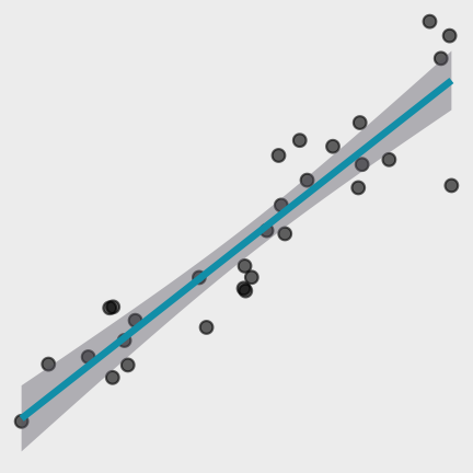
A low dimensional description of a higher dimensional data set.
Models

Data

![]()
Model Function
Models
What is the model function?
Data
Model Function
Models
What uncertainty is associated with it?
Data
Model Function
Models
What are the residuals?
Data
Model Function
Models
What are the predictions?
Data
Model Function
What makes an algorithm "good"?
So many... which one is "best"?
Statistical modeling is an extension of hypothesis testing.
Statistical modeling is an extension of hypothesis testing. Statisticians want to test hypotheses about nature. They do this by formulating those hypotheses as models and then testing the models against data.
At one level, models embed hypotheses like Sale_Price depends on Gr_Liv_Area." We use the model to test whether these hypotheses agree with the data. At another level, the model is a hypothesis and we test how well it comports with the data.
If the model passes the tests, we check to see how much it explains about the data. The best models explain the most. The hope is that we will find a hypothesis that accurately explains the data, and hence reality. In this context, the data is sacred and every model is evaluated by how closely it fits the data at hand.
So statisticians ask questions like, "Is this model a reasonable representation of the world given the data?"
The hypothesis determines
1. Which data to use
2. Which model to use
3. How to assess the model
In other words, statisticians use a model to test the hypotheses in the model. The hypotheses dictate:
- Which data to use
- Which model to use
- How to assess the model, e.g. Does it perform better than the null model according to a well-established, non-generalizable statistical test custom made for the assessment?
This is an important starting place for Machine Learning, because the first thing you need to know about Machine Learning is that Machine Learning is nothing like Hypothesis Testing.


Goal of Machine Learning
Goal of Machine Learning
generate accurate predictions
Goal of Machine Learning
🔮 generate accurate predictions
lm()
lm_ames <- lm(Sale_Price ~ Gr_Liv_Area, data = ames)lm_ames#> #> Call:#> lm(formula = Sale_Price ~ Gr_Liv_Area, data = ames)#> #> Coefficients:#> (Intercept) Gr_Liv_Area #> 13289.6 111.7So let's start with prediction. To predict, we have to have two things: a model to generate predictions, and data to predict
Step 1: Train the model


Specify a model with parsnip
1. Pick a model
2. Set the engine
3. Set the mode (if needed)
Specify a model with parsnip
decision_tree() %>% set_engine("C5.0") %>% set_mode("classification")Specify a model with parsnip
nearest_neighbor() %>% set_engine("kknn") %>% set_mode("regression")To specify a model with parsnip
1. Pick a model
2. Set the engine
3. Set the mode (if needed)
linear_reg()
Specifies a model that uses linear regression
linear_reg(mode = "regression", penalty = NULL, mixture = NULL)linear_reg()
Specifies a model that uses linear regression
linear_reg( mode = "regression", # "default" mode, if exists penalty = NULL, # model hyper-parameter mixture = NULL # model hyper-parameter)To specify a model with parsnip
1. Pick a model
2. Set the engine
3. Set the mode (if needed)
set_engine()
Adds an engine to power or implement the model.
lm_spec %>% set_engine(engine = "lm", ...)To specify a model with parsnip
1. Pick a model
2. Set the engine
3. Set the mode (if needed)
set_mode()
Sets the class of problem the model will solve, which influences which output is collected. Not necessary if mode is set in Step 1.
lm_spec %>% set_mode(mode = "regression")Your turn 1
Write a pipe that creates a model that uses lm() to fit a linear regression. Save it as lm_spec and look at the object. What does it return?
Hint: you'll need https://www.tidymodels.org/find/parsnip/
03:00
lm_spec <- linear_reg() %>% # Pick linear regression set_engine(engine = "lm") # set enginelm_spec#> Linear Regression Model Specification (regression)#> #> Computational engine: lmfit()
Train a model by fitting a model. Returns a {parsnip} model fit.
fit(lm_spec, Sale_Price ~ Gr_Liv_Area, data = ames)fit()
Train a model by fitting a model. Returns a {parsnip} model fit.
fit( model = lm_spec, # parsnip model Sale_Price ~ Gr_Liv_Area, # a formula data = ames # data frame)Your turn 2
Double check. Does
lm_fit <- fit(lm_spec, Sale_Price ~ Gr_Liv_Area, data = ames)lm_fitgive the same results as
lm(Sale_Price ~ Gr_Liv_Area, data = ames)02:00
lm_fit#> parsnip model object#> #> Fit time: 1ms #> #> Call:#> stats::lm(formula = Sale_Price ~ Gr_Liv_Area, data = data)#> #> Coefficients:#> (Intercept) Gr_Liv_Area #> 13289.6 111.7lm(Sale_Price ~ Gr_Liv_Area, data = ames)#> #> Call:#> lm(formula = Sale_Price ~ Gr_Liv_Area, data = ames)#> #> Coefficients:#> (Intercept) Gr_Liv_Area #> 13289.6 111.7data (x, y) + model = fitted model
Step 1: Train the model
Step 2: Make predictions
predict()
Use a fitted model to predict new y values from data. Returns a tibble.
predict(lm_fit, new_data = ames)predict()
Use a fitted model to predict new y values from data. Returns a tibble.
predict( object = lm_fit, # fitted parsnip model new_data = ames # data frame)#> # A tibble: 2,930 x 1#> .pred#> <dbl>#> 1 198255.#> 2 113367.#> 3 161731.#> 4 248964.#> 5 195239.#> 6 192447.#> 7 162736.#> 8 156258.#> 9 193787.#> 10 214786.#> # … with 2,920 more rowsPredictions
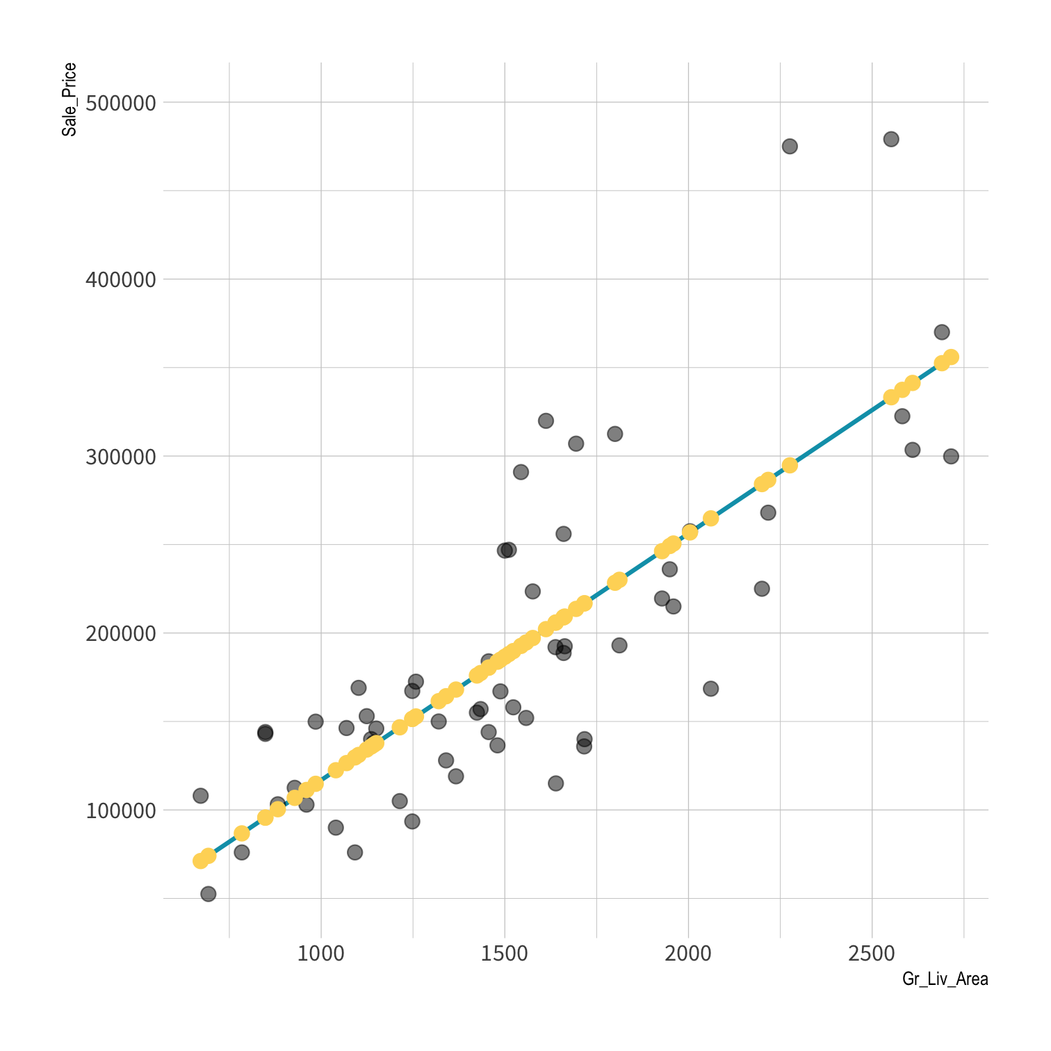
Your turn 3
Fill in the blanks. Use predict() to:
- Use your linear model to predict sale prices: save the tibble as
price_pred. - Add a pipe and use
mutate()to add a column with the observed sale prices; name ittruth.
lm_fit <- fit(lm_spec, Sale_Price ~ Gr_Liv_Area, data = ames)

price_pred <-        %>%
  predict(new_data = ames) %>%


price_pred
03:00
lm_fit <- fit(lm_spec, Sale_Price ~ Gr_Liv_Area, data = ames)price_pred <- lm_fit %>% predict(new_data = ames) %>% mutate(truth = ames$Sale_Price)price_pred#> # A tibble: 2,930 x 2#> .pred truth#> <dbl> <int>#> 1 198255. 215000#> 2 113367. 105000#> 3 161731. 172000#> 4 248964. 244000#> 5 195239. 189900#> 6 192447. 195500#> 7 162736. 213500#> 8 156258. 191500#> 9 193787. 236500#> 10 214786. 189000#> # … with 2,920 more rowsdata (x, y) + model = fitted model
data (x, y) + model = fitted model
data (x) + fitted model = predictions
Goal of Machine Learning
🔮 generate accurate predictions
Goal of Machine Learning
🎯 generate accurate predictions
Now we have predictions from our model. What can we do with them? If we already know the truth, that is, the outcome variable that was observed, we can compare them!
Axiom
Better Model = Better Predictions (Lower error rate)
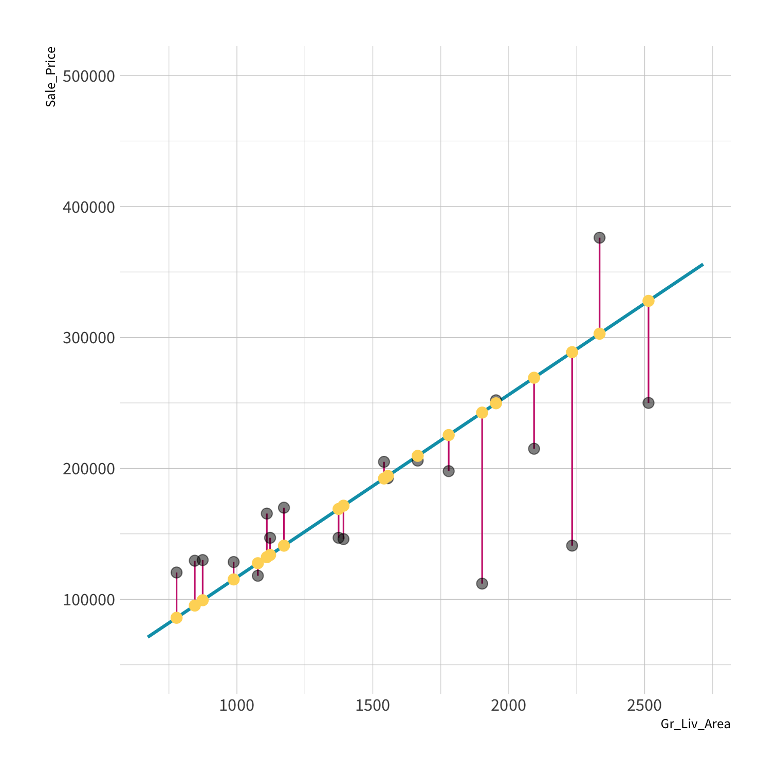
Predictions
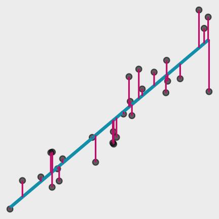
Residuals
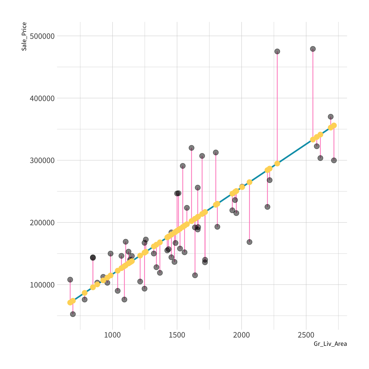
Residuals
The difference between the predicted and observed values.
^yi−yi
refers to a single residual. Since residuals are errors, the sum of the errors would be a good measure of total error except for two things. What's one of them?
Consider
What could go wrong?
n∑i=1^yi−yi
First, the sum would increase every time we add a new data point. That means models fit on larger data sets would have bigger errors than models fit on small data sets. That makes no sense, so we work with the mean error.
Consider
What could go wrong?
1nn∑i=1^yi−yi
What else makes this an insufficient measure of error?
Positive and negative residuals would cancel each other out. We can fix that by taking the absolute value of each residual...
Consider
What could go wrong?
1nn∑i=1|^yi−yi|
Mean Absolute Error
...but absolute values are hard to work with mathematically. They're not differentiable at zero. That's not a big deal to us because we can use computers. But it mattered in the past, and as a result statisticians used the square instead, which also penalizes large residuals more than smaller residuals. The square version also has some convenient throretical properties. It's the standard deviation of the residuals about zero. So we will use the square.
Consider
What could go wrong?
1nn∑i=1(^yi−yi)2
If you take the square, then to return things to the same units as the residuals, you have the the root mean square error.
Consider
What could go wrong?
⎷1nn∑i=1(^yi−yi)2
Root Mean Squared Error
RMSE
Root Mean Squared Error - The standard deviation of the residuals about zero.
⎷1nn∑i=1(^yi−yi)2


rmse()
Calculates the RMSE based on two columns in a dataframe:
The truth: yi
The predicted estimate: ^yi
rmse(data, truth, estimate)lm_fit <- fit(lm_spec, Sale_Price ~ Gr_Liv_Area, data = ames)price_pred <- lm_fit %>% predict(new_data = ames) %>% mutate(price_truth = ames$Sale_Price)rmse(price_pred, truth = price_truth, estimate = .pred)#> # A tibble: 1 x 3#> .metric .estimator .estimate#> <chr> <chr> <dbl>#> 1 rmse standard 56505.Step 1: Train the model
Step 2: Make predictions
Step 3: Compute metrics
data (x, y) + model = fitted model
data (x, y) + model = fitted model
data (x) + fitted model = predictions
data (x, y) + model = fitted model
data (x) + fitted model = predictions
data (y) + predictions = metrics
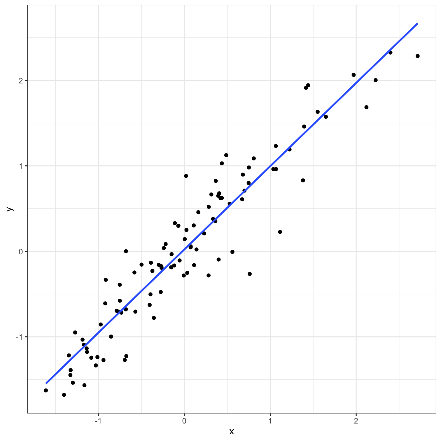
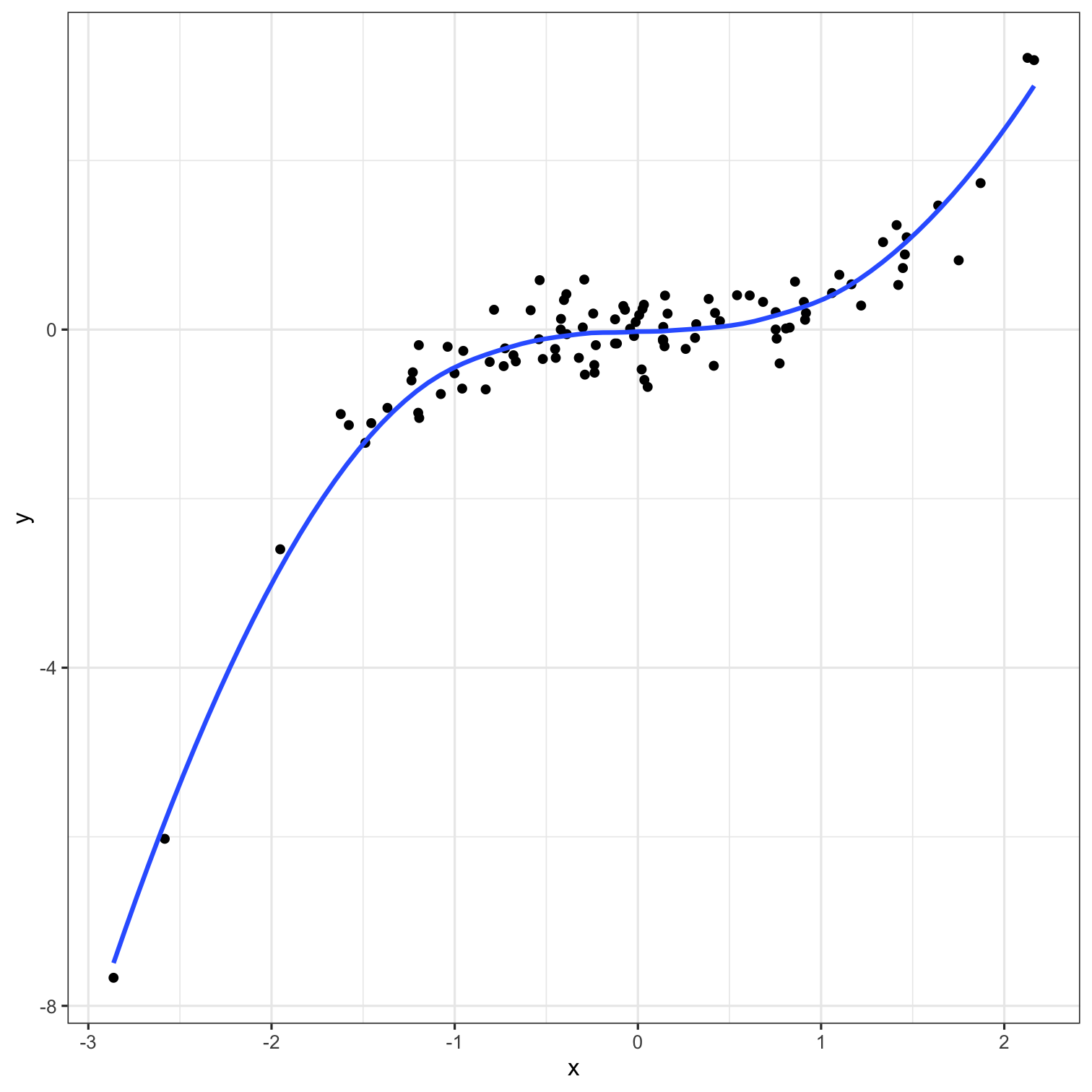
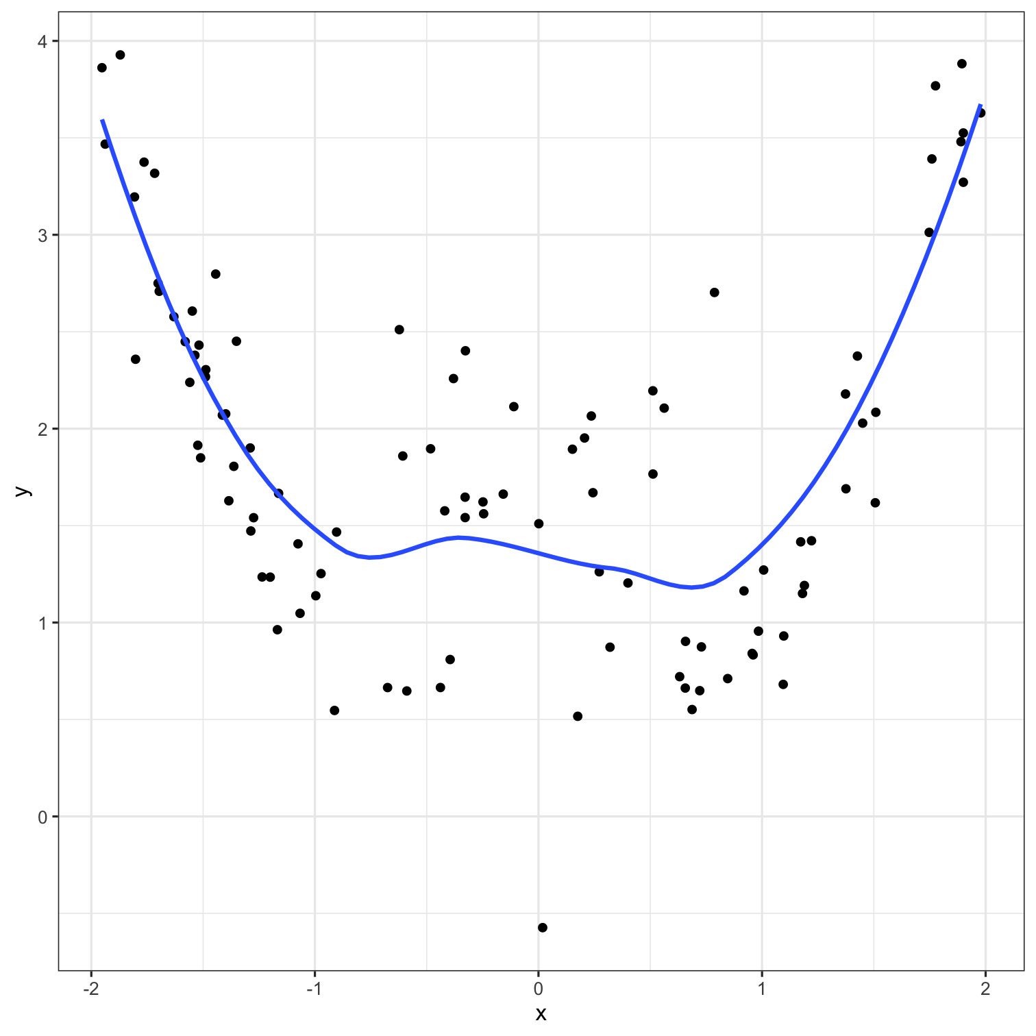
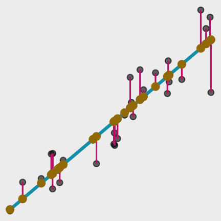
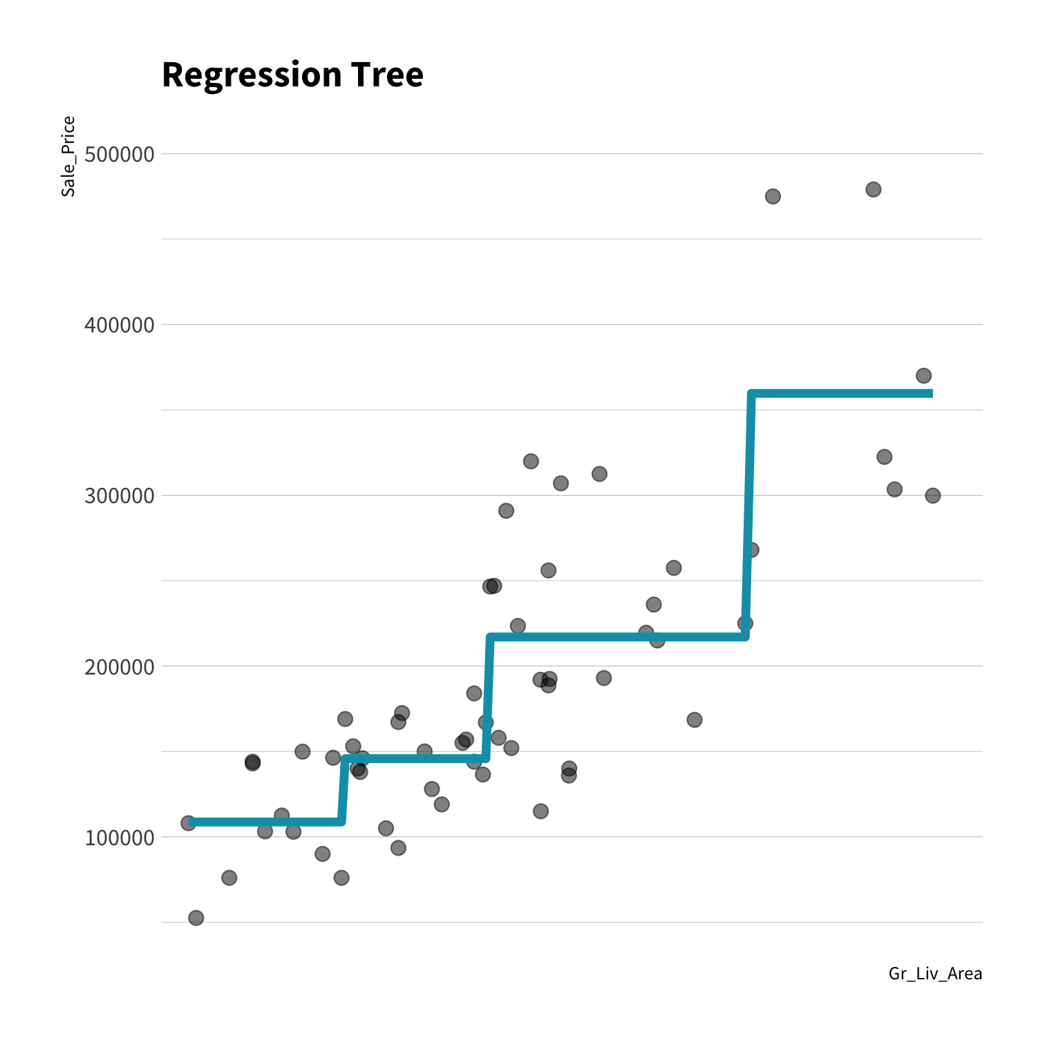
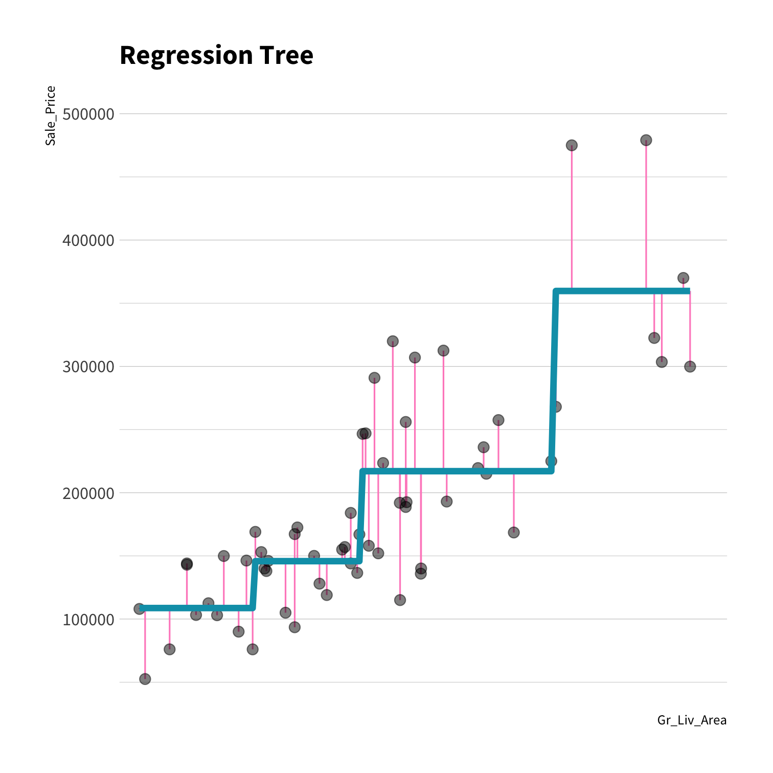
A model doesn't have to be a straight line!
Do you trust it?
Overfitting
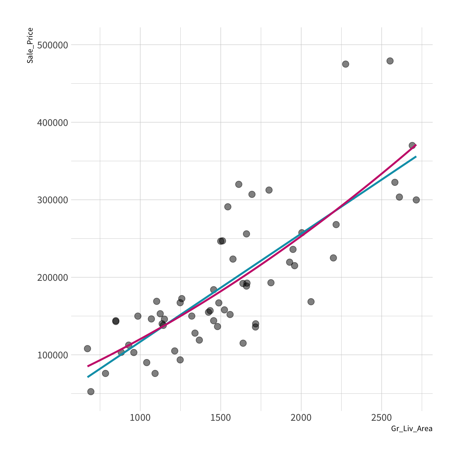
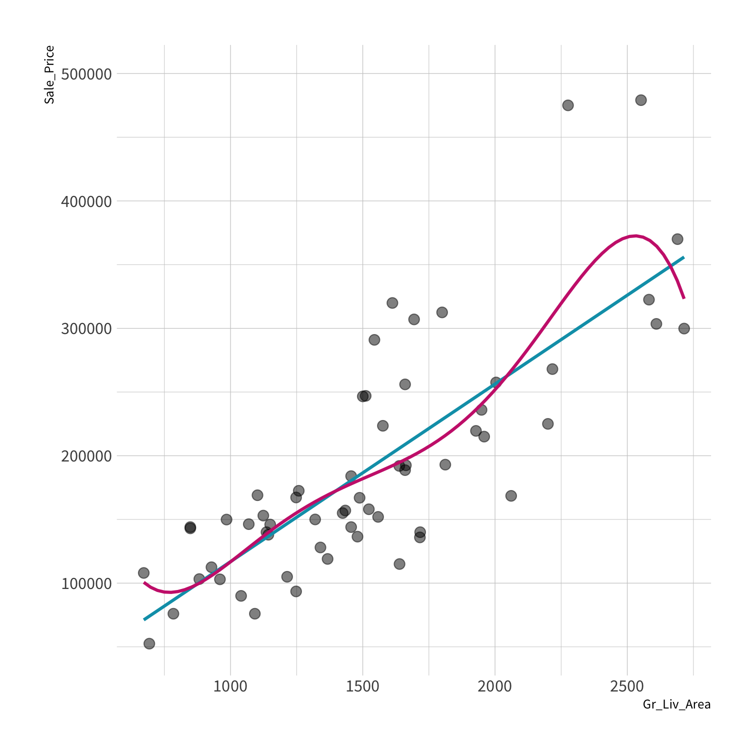

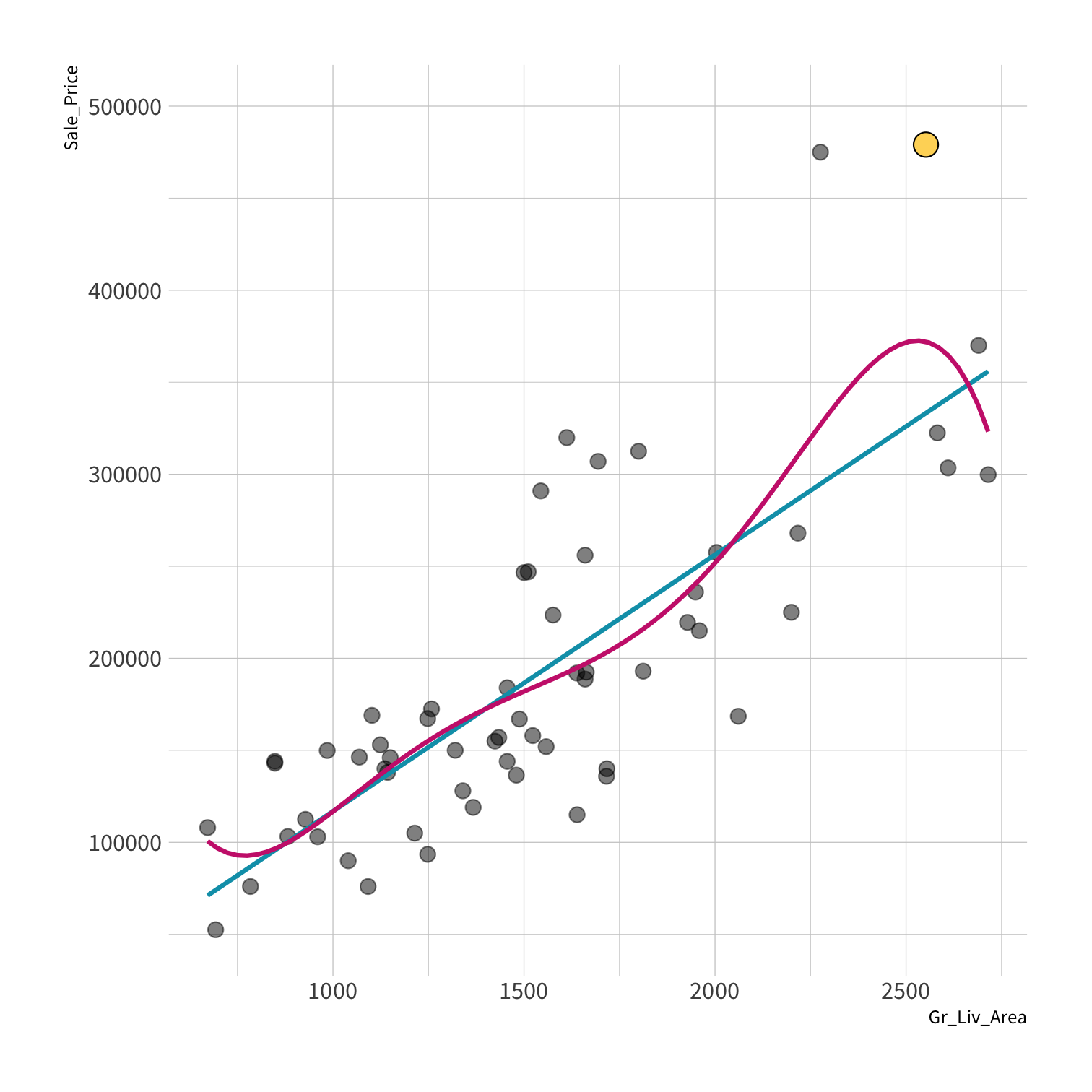
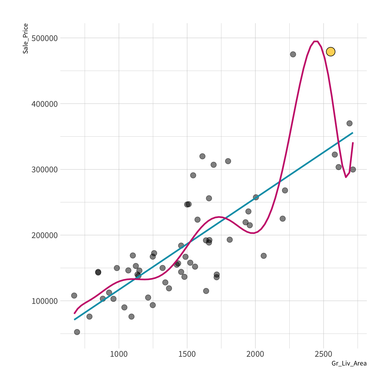
Your turn 4
Discuss in the chat which model:
- Has the smallest residuals
- Will have lower prediction error. Why?
02:00
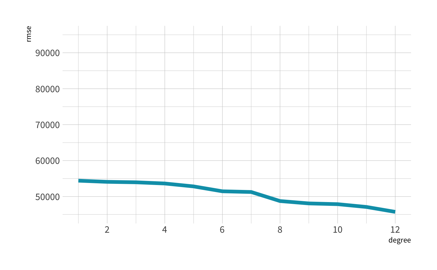
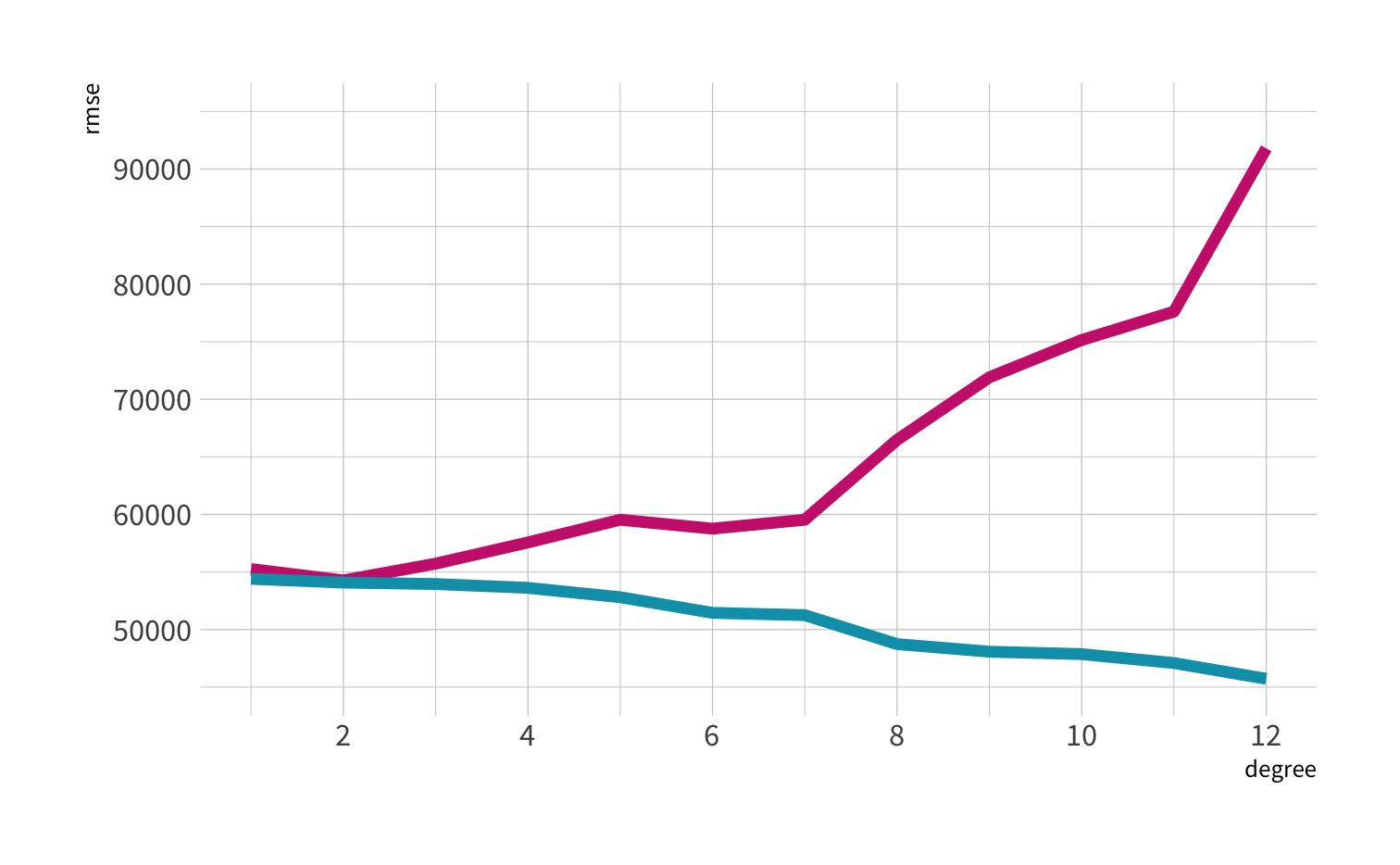
Residuals - as the polynomial increases, the residuals get smaller and smaller.
BUT, the out of sample prediction error gets larger and larger.
Axiom
The best way to measure a model's performance at predicting new data is to predict new data.
Goal of Machine Learning
Goal of Machine Learning
🔨 construct models that
Goal of Machine Learning
🔨 construct models that
🎯 generate accurate predictions
Goal of Machine Learning
🔨 construct models that
🎯 generate accurate predictions
🆕 for future, yet-to-be-seen data
Goal of Machine Learning
🔨 construct models that
🎯 generate accurate predictions
🆕 for future, yet-to-be-seen data
Max Kuhn & Kjell Johnston, http://www.feat.engineering/
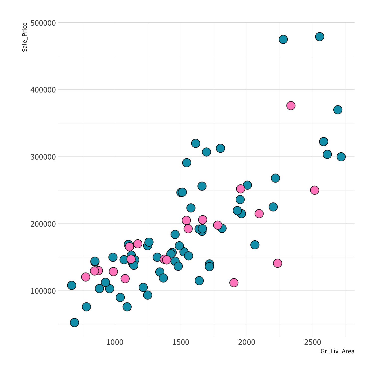
But need new data...
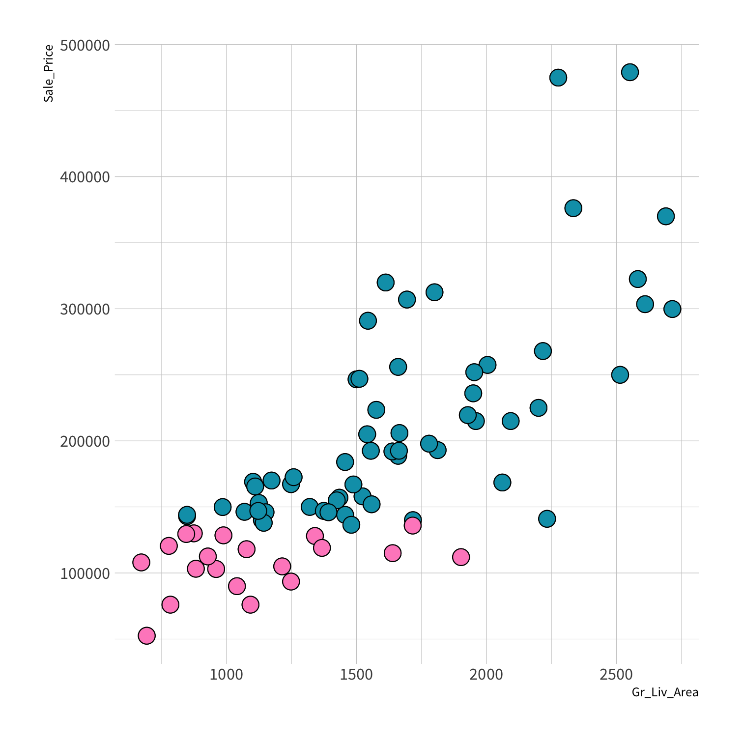
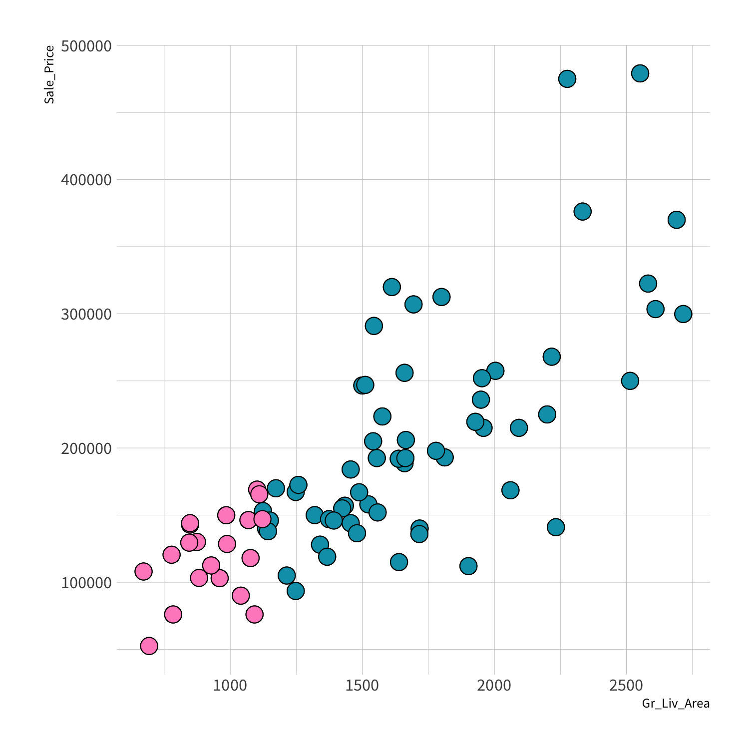
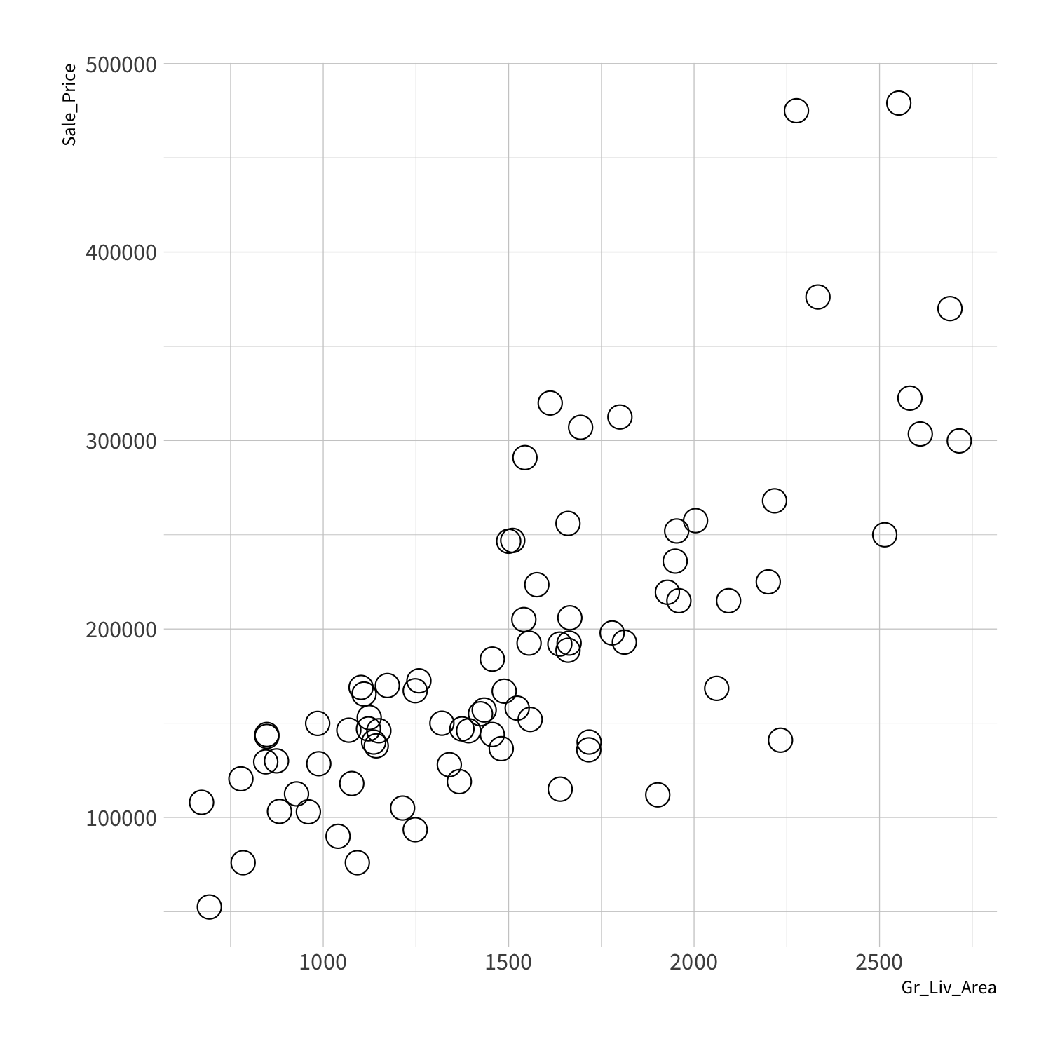
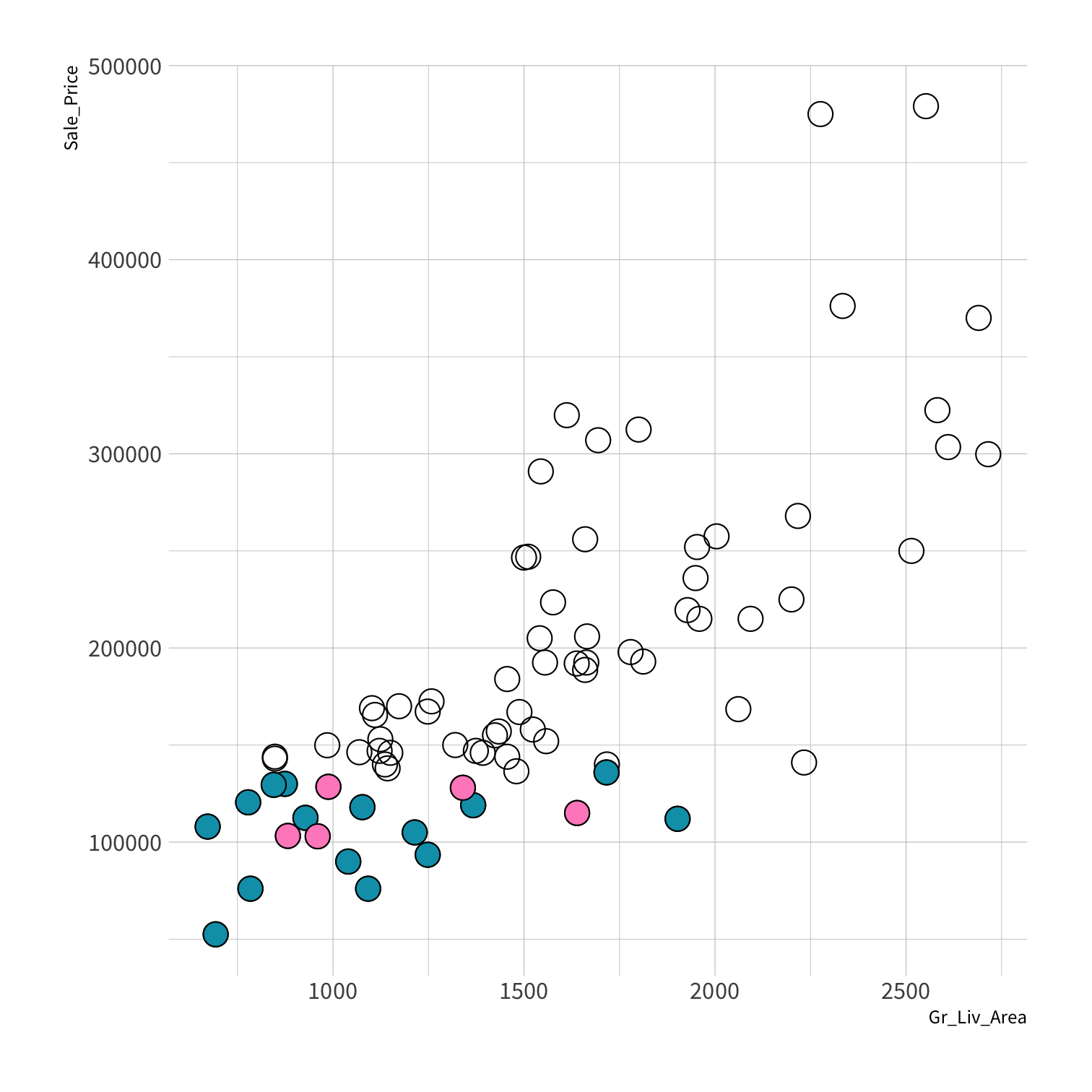
Method #1
The holdout method

We refer to the group for which we know the outcome, and use to develop the algorithm, as the training set. We refer to the group for which we pretend we don’t know the outcome as the test set.
initial_split()
"Splits" data randomly into a single testing and a single training set.
initial_split(data, prop = 3/4)ames_split <- initial_split(ames, prop = 0.75)ames_split#> <Analysis/Assess/Total>#> <2198/732/2930>data splitting
training() and testing()
Extract training and testing sets from an rsplit
training(ames_split)testing(ames_split)train_set <- training(ames_split) train_set#> # A tibble: 2,198 x 74#> MS_SubClass MS_Zoning Lot_Frontage Lot_Area Street Alley Lot_Shape #> <fct> <fct> <dbl> <int> <fct> <fct> <fct> #> 1 One_Story_1946_… Residential… 141 31770 Pave No_All… Slightly_…#> 2 One_Story_1946_… Residential… 81 14267 Pave No_All… Slightly_…#> 3 Two_Story_1946_… Residential… 74 13830 Pave No_All… Slightly_…#> 4 Two_Story_1946_… Residential… 78 9978 Pave No_All… Slightly_…#> 5 One_Story_PUD_1… Residential… 41 4920 Pave No_All… Regular #> 6 One_Story_PUD_1… Residential… 43 5005 Pave No_All… Slightly_…#> 7 Two_Story_1946_… Residential… 60 7500 Pave No_All… Regular #> 8 Two_Story_1946_… Residential… 75 10000 Pave No_All… Slightly_…#> 9 One_Story_1946_… Residential… 0 7980 Pave No_All… Slightly_…#> 10 Two_Story_1946_… Residential… 63 8402 Pave No_All… Slightly_…#> # … with 2,188 more rows, and 67 more variables: Land_Contour <fct>,#> # Utilities <fct>, Lot_Config <fct>, Land_Slope <fct>, Neighborhood <fct>,#> # Condition_1 <fct>, Condition_2 <fct>, Bldg_Type <fct>, House_Style <fct>,#> # Overall_Cond <fct>, Year_Built <int>, Year_Remod_Add <int>,#> # Roof_Style <fct>, Roof_Matl <fct>, Exterior_1st <fct>, Exterior_2nd <fct>,#> # Mas_Vnr_Type <fct>, Mas_Vnr_Area <dbl>, Exter_Cond <fct>, Foundation <fct>,#> # Bsmt_Cond <fct>, Bsmt_Exposure <fct>, BsmtFin_Type_1 <fct>,#> # BsmtFin_SF_1 <dbl>, BsmtFin_Type_2 <fct>, BsmtFin_SF_2 <dbl>,#> # Bsmt_Unf_SF <dbl>, Total_Bsmt_SF <dbl>, Heating <fct>, Heating_QC <fct>,#> # Central_Air <fct>, Electrical <fct>, First_Flr_SF <int>,#> # Second_Flr_SF <int>, Gr_Liv_Area <int>, Bsmt_Full_Bath <dbl>,#> # Bsmt_Half_Bath <dbl>, Full_Bath <int>, Half_Bath <int>,#> # Bedroom_AbvGr <int>, Kitchen_AbvGr <int>, TotRms_AbvGrd <int>,#> # Functional <fct>, Fireplaces <int>, Garage_Type <fct>, Garage_Finish <fct>,#> # Garage_Cars <dbl>, Garage_Area <dbl>, Garage_Cond <fct>, Paved_Drive <fct>,#> # Wood_Deck_SF <int>, Open_Porch_SF <int>, Enclosed_Porch <int>,#> # Three_season_porch <int>, Screen_Porch <int>, Pool_Area <int>,#> # Pool_QC <fct>, Fence <fct>, Misc_Feature <fct>, Misc_Val <int>,#> # Mo_Sold <int>, Year_Sold <int>, Sale_Type <fct>, Sale_Condition <fct>,#> # Sale_Price <int>, Longitude <dbl>, Latitude <dbl>Pop quiz!
Now that we have training and testing sets...
Pop quiz!
Now that we have training and testing sets...
Which data set do you think we use for fitting?
Pop quiz!
Now that we have training and testing sets...
Which data set do you think we use for fitting?
Which do we use for predicting?
Step 1: Train the model
Step 2: Make predictions
Step 3: Compute metrics
Step 3: Compute metrics
Step 1: Split the data
Step 2: Train the model
Step 3: Make predictions
Step 4: Compute metrics
Your turn 5
Use initial_split(), training(), testing(), lm() and rmse() to:
Split ames into training and test sets. Save the rsplit!
Extract the training data. Fit a linear model to it. Save the model!
Measure the RMSE of your model with your test set.
set.seed(100)

ames_split  <-
ames_train  <-
ames_test   <-

lm_fit <- fit(lm_spec,
              Sale_Price ~ Gr_Liv_Area,
              data = ames_train)

price_pred <- lm_fit %>%
  predict(new_data = ames_test) %>%
  mutate(price_truth =                     )

rmse(price_pred, truth = price_truth,
     estimate =      )
05:00
set.seed(100)ames_split <- initial_split(ames)ames_train <- training(ames_split)ames_test <- testing(ames_split)lm_fit <- fit(lm_spec, Sale_Price ~ Gr_Liv_Area, data = ames_train)price_pred <- lm_fit %>% predict(new_data = ames_test) %>% mutate(price_truth = ames_test$Sale_Price)rmse(price_pred, truth = price_truth, estimate = .pred)#> # A tibble: 1 x 3#> .metric .estimator .estimate#> <chr> <chr> <dbl>#> 1 rmse standard 59310.RMSE = 59310.14; compare to 56504.88 when using full data
Training RMSE = 55539.85
Training RMSE = 55539.85
Testing RMSE = 59310.14
old data (x, y) + model = fitted model
old data (x, y) + model = fitted model
new data (x) + fitted model = predictions
old data (x, y) + model = fitted model
new data (x) + fitted model = predictions
new data (y) + predictions = metrics
Consider
How much data should you set aside for testing?
Consider
How much data should you set aside for testing?
If testing set is small, performance metrics may be unreliable.
Consider
How much data should you set aside for testing?
If testing set is small, performance metrics may be unreliable.
If training set is small, model fit may be poor.
Stratified sampling

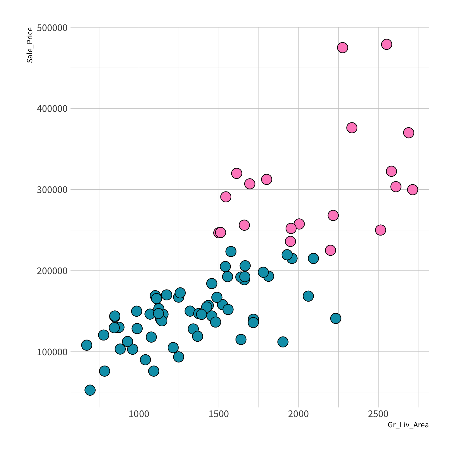
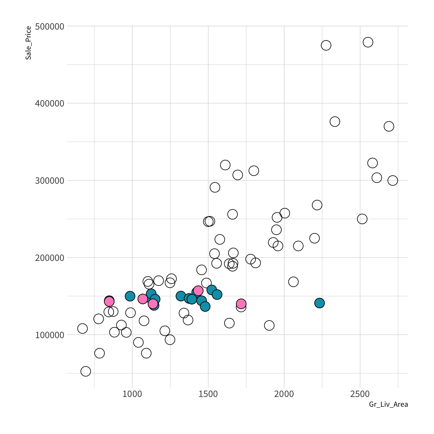
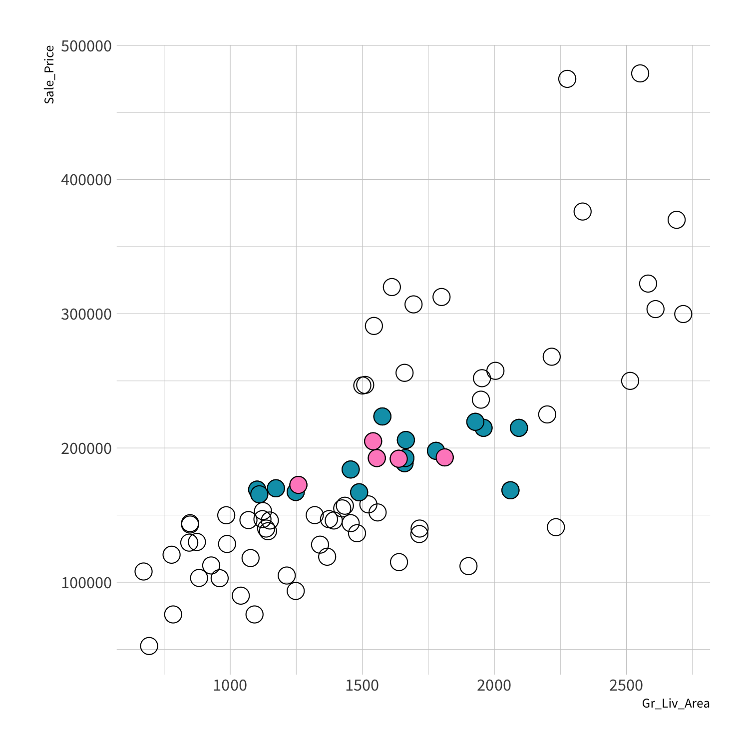
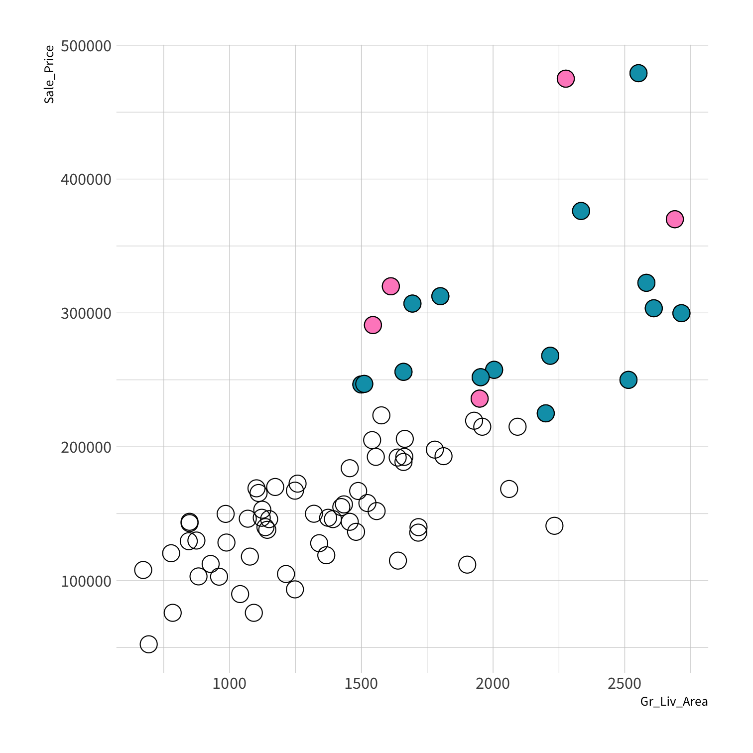
set.seed(100) # Important!ames_split <- initial_split(ames, strata = Sale_Price, breaks = 4)ames_train <- training(ames_split)ames_test <- testing(ames_split)lm_fit <- fit(lm_spec, Sale_Price ~ Gr_Liv_Area, data = ames_train)price_pred <- lm_fit %>% predict(new_data = ames_test) %>% mutate(price_truth = ames_test$Sale_Price)rmse(price_pred, truth = price_truth, estimate = .pred)decision_tree()
Specifies a decision tree model
decision_tree(tree_depth = NULL, min_n = NULL, cost_complexity = NULL)Your turn 6
Write a pipe to create a model that uses the {rpart} package to fit a regression tree and calculate the RMSE.
Compare to the lm() model. Which is better?
Hint: you'll need https://www.tidymodels.org/find/parsnip/
05:00
set.seed(100) # Important!ames_split <- initial_split(ames, strata = Sale_Price, breaks = 4)ames_train <- training(ames_split)ames_test <- testing(ames_split)lm_spec <- linear_reg() %>% set_engine("lm") %>% set_mode("regression")lm_fit <- fit(lm_spec, Sale_Price ~ Gr_Liv_Area, data = ames_train)price_pred <- lm_fit %>% predict(new_data = ames_test) %>% mutate(price_truth = ames_test$Sale_Price)lm_rmse <- rmse(price_pred, truth = price_truth, estimate = .pred)rt_spec <- decision_tree() %>% set_engine("rpart") %>% set_mode("regression")dt_fit <- fit(rt_spec, Sale_Price ~ Gr_Liv_Area, data = ames_train)price_pred <- dt_fit %>% predict(new_data = ames_test) %>% mutate(price_truth = ames_test$Sale_Price)dt_rmse <- rmse(price_pred, truth = price_truth, estimate = .pred)lm_rmse#> # A tibble: 1 x 3#> .metric .estimator .estimate#> <chr> <chr> <dbl>#> 1 rmse standard 57734.dt_rmse#> # A tibble: 1 x 3#> .metric .estimator .estimate#> <chr> <chr> <dbl>#> 1 rmse standard 59716.nearest_neighbor()
Specifies a KNN model
nearest_neighbor(neighbors = 1)Your turn 7
Write another pipe to create a model that uses the {kknn} package to fit a K nearest neighbors model. Calculate the RMSE to compare to our other models that use the same formula.
Hint: you'll need https://www.tidymodels.org/find/parsnip/
05:00
knn_spec <- nearest_neighbor() %>% set_engine(engine = "kknn") %>% set_mode("regression")knn_fit <- fit(knn_spec, Sale_Price ~ Gr_Liv_Area, data = ames_train)price_pred <- knn_fit %>% predict(new_data = ames_test) %>% mutate(price_truth = ames_test$Sale_Price)knn_rmse <- rmse(price_pred, truth = price_truth, estimate = .pred)lm_rmse#> # A tibble: 1 x 3#> .metric .estimator .estimate#> <chr> <chr> <dbl>#> 1 rmse standard 57734.dt_rmse#> # A tibble: 1 x 3#> .metric .estimator .estimate#> <chr> <chr> <dbl>#> 1 rmse standard 59716.knn_rmse#> # A tibble: 1 x 3#> .metric .estimator .estimate#> <chr> <chr> <dbl>#> 1 rmse standard 61103.Prediction

Tidy Data Science with the Tidyverse and Tidymodels
W. Jake Thompson
https://tidyds-2021.wjakethompson.com · https://bit.ly/tidyds-2021
Tidy Data Science with the Tidyverse and Tidymodels is licensed under a Creative Commons Attribution 4.0 International License.